13  Horizon architecture

Each soil horizon may include any or all of the following major components:

• Solid fraction
  • Fine earth
  • Fragments
  • Artefacts
• Biological fraction
  • Fine organic matter
  • Coarse organic matter
  • Living plant roots
• Liquid fraction
• Void space fraction
  • Voids
  • Pores
    • Macropores
    • Micropores

These fractions can be communicated as compositional percentage by volume, adding to 100%. The fine-earth fraction also has its own compositional data based on finer divisions of the < 2 mm fraction (see Chapter 15). Volumetric water content is best determined in the laboratory, and so is not described further.

complicated exploding pie chart or similar goes here

Soil horizon architecture includes both composition and the physical arrangement of the above components.

13.1 Structure

Structure refers to the physical arrangement of the fine-earth fraction (mineral materials < 2 mm). Structure is determined by mineralogy, chemistry, the action of soil biota and land use history. Structure may be pedogenic, geogenic, or human-induced (Anderson et al. 2024).

• To assess the structure in an E or P2 type profile (Table 10.3), insert a spade horizontally near the base of the horizon and push down on the handle, levering out a section of soil. Drop the spade blade with the soil, approximately 0.3 m onto a hard surface, e.g., the blade of another spade. Remove major roots that bind the mass together and again note the attributes of the newly produced solids. Note that this procedure will not necessarily disaggregate very moist or wet soils.
• For smaller exposures (P1, C1, C2), remove a handful of soil from the extracted horizon and carefully disaggregate the soil mass to segregate all peds. Do not destroy peds to create fragments, or disaggregate existing apedal material. Note the attributes of the solids as instructed below. For smaller exposures, also use a spade to extract surface material so that at least the topmost horizon can be assessed in detail.
• Assessing structure is generally impossible for A augered profiles, as the extraction method destroys it. However, the surface horizon should still be extracted with a spade and assessed if possible.
• Structure of hard layers may need to be assessed in place, or by careful removal of individual units, and will usually require an E or P2 type profile.

Sieving or direct measurement of solids may help estimate size. Weighing, or filling volumetric containers, may help estimate abundance of different classes of solids.

13.1.1 Structure type

Structural development can be controlled by different processes depending on vertical position within the profile and land use history. Optionally, record the dominant structural unit type using Table 13.1. Where not recorded, it should be assumed that the formation mechanism is P.

Table 13.1: Type of structural development

Code	Name	Description
P	Pedogenic	Structural units meet the definition of natural soil peds and occur largely within the solum
G	Geogenic	Structural units are inherited from parent materials that have undergone limited weathering e.g. bedding planes, and occur largely below the solum
A	Anthrogenic	Structural units have been induced by human activity, usually within the solum and most commonly in surface horizons
U	Unknown	Type of structural development could not be determined with confidence

13.1.2 Structure development

Degree of structural development provides information about permeability, in concert with texture and firmness.

For rapid assessment, record degree of overall structural development once per horizon using Table 13.2. For routine or detailed assessment, record degree of development for each nested structural unit observed (if more than one is seen; see Section 13.1.4.1).

Table 13.2: Degree of structural development

Code	Name	Description
G	Single grain	Material is structureless and incoherent, with more than 85% by weight of discrete primary particles ranging in size from sand to very coarse gravel.
V	Massive	Material is structureless but coherent, with no fissures at spacings of less than 200 mm
W	Weak	Material where 15-25% of the material comprises coherent structural units
M	Moderate	Material where 25-75% of the material comprises coherent structural units
S	Strong	Material where >75% of the material comprises coherent structural units

13.1.3 Structure shape

Where distinct structural units can be identified (development types W, M, S), record their dominant shape using Table 13.3.

Table 13.3: Structural shapes and identifying characteristics (adapted from Milne et al. (1995), IUSS Working Group WRB (2022), and Soil and Terrain (2009))

Code	Name	Description	Orientation
AB	Angular blocky	Bounded by relatively flat smooth, roughly equal faces number of faces variable most vertices angular usually much accommodation to the faces of surrounding aggregates	None
BL	Blocky	Bounded by undulating rough faces number of faces variable many vertices rounded limited accommodation to the faces of surrounding aggregates	None
PH	Polyhedral	Bounded by relatively flat smooth, unequal faces more than six faces; most vertices angular usually much accommodation to the faces of surrounding aggregates re-entrant angles between adjoining faces - peds ‘lock’ together	None
SR	Spheroidal	bounded by curved or very irregular faces; limited accommodation to the faces of surrounding aggregates sometimes with many visible pores	None
LT	Lenticular	Bounded by curved faces overlapping, lens-shaped aggregates generally parallel to the soil surface that are thick at the centre and taper toward the edges usually much accommodation to the faces of surrounding aggregates	Horizontal or shallow angle
PM	Prismatic	Bounded by relatively flat faces vertically elongated units with angular vertices and flat tops much accommodation to the faces of surrounding aggregates	Vertical
CO	Columnar	Bounded by relatively flat faces; vertically elongated units with angular to rounded vertices and rounded (domed) tops	Vertical
PL	Platy	Bounded by relatively flat horizontal faces much accommodation to the faces of surrounding aggregates	Horizontal
LF	Lentiform	Bounded by curved faces overlapping, lens-shaped aggregates generally parallel to the soil surface that are thick at the centre and taper toward the edges usually much accommodation to the faces of surrounding aggregates	Horizontal or shallow-angle
WL	Wedge-like	Bounded by flat faces; interlocking wedges or lenses that terminate in pronounced angular vertices; ends of vertices may be missing; much accommodation to the faces of surrounding aggregates	Horizontal

add diagrams

Note 13.1: Shorthand terms for structural units

Some pedogenic structural terms that don’t seem to fit into the above schema are still in common use.

• Crumb structure: a very fine structure seen in many silty to loamy horizons. The appearance is as of breadcrumbs, with 0.5-2 mm rounded peds loosely to firmly packed, depending on depth and drainage. Larger weak subangular blocky structures in well-drained allophanic soils almost always break down into moderately or strongly developed crumb structure.
• Nut structure: a larger version of crumb, usually on the order of 5-20 mm in diameter, often encased in a network of grass roots. Nut structures are more common in topsoils but can also occur in well-drained loamy subsoils.

Both structures are more correctly described as type P with SR shape. ‘Crumbs’ have a size range of about 1 ± 0.5 mm and ‘nuts’ are about 15 ± 10 mm. Their use as a shorthand description is convenient, but the terms should not be used in databases because they conflate size and shape in a way that the modern schemas seek to avoid.

Similarly, the terms ‘clod’ and ‘fragment’, previously used to signify tillage-induced structures greater and less than 100 mm in length respectively, also conflate size and shape. These should more correctly be described as type A structures with (usually) BL or PH shape.

13.1.4 Structure size

Record the median length of the structural units observed, along their longest axis. Record in mm with a range estimate, e.g. 25 ± 2 mm.

For rapid assessment, the dominant size may be recorded consistent with the NZSC Functional Horizon convention - (Table 20.15, C for Coarse or F for Fine).

13.1.4.1 Nesting units

Structural units are commonly nested, with large structures breaking down to smaller ones that may also be a different type and shape. For highly detailed descriptions, multiple sets of nesting peds may be described in terms of their development, shape and size.

For example, S PR 80 ± 10 parting to M BL 20 ± 2.

13.2 Fragments

Fragments in soil horizons (> 2 mm) provide information about soil development, particularly mode of emplacement in depositional soils. They also restrict the soil’s water holding capacity, and when large and common enough can restrict land use and management practices.

For very rapid assessment, estimate total fragment abundance (rocks and non-rock materials as well as any artefacts) as an integer percentage, recording 0% when confirming absence.

13.2.1 Rock fragments

Rock fragments are soil mineral particles > 2 mm. For rapid assessment, estimate total rock fragment abundance as an integer percentage, recording 0% when confirming absence.

For routine assessment, estimate abundance of small, medium and large rock fragments separately (Table 13.4). Optionally, append dominant lithology class of each size fraction using Table 24.2 and shape using Table 13.5.

Example: 60% M (Hs R), 5% L (Hs R) for a fluvial deposit dominated by waterworn greywacke cobbles with a few boulders.

For detailed assessment, estimate abundance, lithology, and shape for each of the ‘gravel’ classes in Table 21.1.

Table 13.4: Fragment size classes for routine assessment

Code	Name	Size range (mm)
S	Small	2 - 60
M	Medium	60 - 200
L	Large	> 200

Table 13.5: Coarse fragment shape classes

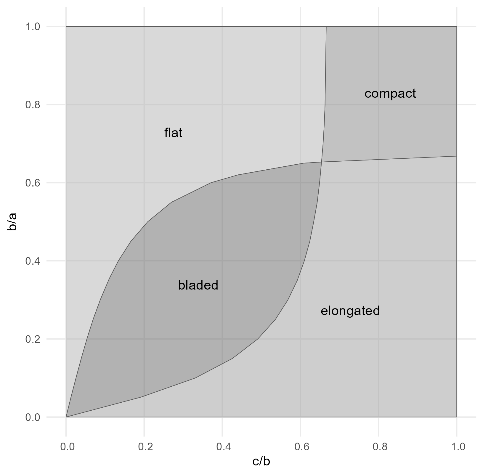
Code	Name	Description
R	Rounded	Rock fragments considerably smoothed by transport processes
A	Angular	Rock fragments with little smoothing by transport processes
M	Mixed	Both rounded and angular fragments mixed together

13.2.2 Natural fragments

Biologically-derived coarse materials can alter the soil’s water holding capacity and other parameters just as rock fragments can, although in general they can themselves hold more water. They will also break down faster.

Where present in significant amounts, for rapid assessment record total percentage of natural non-rock fragments. For routine assessment record percentage abundance by type for small, medium and large sizes (Table 13.4) using Table 13.6.

Table 13.6: Non-rock fragment types

Code	Name	Description
S	Shell	Seashells or chitinous material
B	Bone	Skeletal fragments
T	Timber	Dead wood from trees and shrubs, coarse roots
C	Charcoal	Burnt organic materials
G	Gum	Kauri gum

13.2.3 Artefacts

Artefacts can both function like rock fragments and signify strong human influence on the soil profile.

Where present in significant amounts, for rapid assessment record total percentage of artefacts. For routine assessment record percentage abundance by type for small, medium and large sizes (Table 13.4) using Table 13.7.

Where further details are required, describe the materials present in free-text notes.

Table 13.7: Artefact types

Code	Name	Description
As	Asphalt	Asphalt and other bitumen-containing materials
Br	Brick	Fired clay building materials, usually unglazed
Cr	Ceramic	Fired clay objects, usually glazed
Ce	Concrete	Concrete materials, cements
Gl	Glass	Fragments from windows, containers, etc
Pl	Plastics	Artificial polymers (non-textile)
Tn	Textiles - natural	Fabrics and carpets made from e.g. wool
Tx	Textiles - artificial	Fabrics derived from or dominated by plastics
Mt	Metals	Refined ore products
Ms	Mine Spoil	Materials leftover from ore processing activities
Ws	Wastes	Other domestic or commercial rubbish

13.2.4 Plastics

More specific and detailed assessment of macroplastics may be desired for certain applications. The following optional schema is adapted from Weber (2022). For the size fractions in Table 13.4, one may describe abundance by volume plus any or all of the origin, fixation, shape, and degradation codes supplied below. Colour may also be described using common terms. Smaller plastic fragments (microplastics) may require sampling and laboratory analysis.

Table 13.8: Plastic fragment origin

Code	Name	Description
N	Not verifiable	Designation not possible / uncertain
C	Consumer	Consumer-products (everyday-products) like PET-bottles, SUP bags, packages, signs etc.
A	Agricultural	Agricultural products like mulch film, silage film, straw bale nets, tire wear etc.
I	Industrial	Industrial products like broken pieces of industrial equipment, industrial waste
B	Construction	All plastic materials which were placed in soil for construction and supply purposes (e.g., power cables, geomembranes)

Table 13.9: Plastic fragment fixation

Code	Name	Description
NF	None	Plastic pieces are not included in soil aggregates (no soil aggregates or loose plastic)
SF	Solely	Single plastic pieces are in cooperated into soil aggregates, but others are loose
MF	Moderate	The majority of plastic pieces is in cooperated into soil aggregates, but single are loose
CF	Complete	All plastic pieces are in cooperated into soil aggregates

Table 13.10: Plastic fragment shape

Code	Name	Description
P	Preserved	The original manufactured shape of the object is recognisable
B	Broken	The fragment is recognisable as having been part of a larger object
F	Flat	Tabular or sheet-like
A	Angular	Sharp-edged
R	Rounded	Has edges that are not sharp
S	Spherical	Ball shaped or ovoid

Table 13.11: Plastic fragment degradation

Code	Name	Description
N	Not verifiable	Designation not possible / uncertain
F	Fresh	Fresh plastic pieces with bright colours, unaffected shape, without signs of deterioration (cracks, broken edges, rough surfaces)
I	Incipient alteration	Plastic pieces with incipient deterioration surface such as first cracks, broken edges or roughened/grooved surfaces
D	Degraded	Plastic pieces with clear indications of ageing such as pale colours or yellowing (UV light), strong fragmentation, frayed edges
S	Strongly degraded	Plastic pieces with strong degraded surfaces, faded colours, soft surface, frayed areas or edges

13.3 Roots

Plant roots affect water infiltration and help define the functional horizon topsoil (see Section 20.2.1.1). Their position in the soil profile can also provide information about ped development, particle packing, and the presence of pans. Note that this section does not apply to peats.

13.3.1 Root abundance

Measure abundance by estimating the volumetric abundance of live roots in the visible soil horizon. For roots < 2 mm it may be more practical to sample a cube ~100 mm on a side. When augering for rapid assessment, also use a spade to sample the topsoil.

For rapid assessment, estimate the volume of the whole root mass as integer %, confirming 0 if no roots are observed.

For example: 25% for a healthy pasture topsoil.

For detailed assessment, provide separate estimates for the root size classes in Table 13.12. Record as whole percentages, confirming 0% where no roots are observable in a given size range. The data may be classified using Table 21.3.

Table 13.12: Plant root size classes for detailed assessment

Code	Name	Size range (mm)
F	Fine	< 2
M	Medium	2 - 10
C	Coarse	> 10

For example: F 5%, M 0%, C 2% for a subsoil in a forested area.

13.3.2 Root position

Where abundance is > 0%, record how roots are distributed within the horizon using the codes in Table 13.13. Position may not be reliably observable outside of pits or exposures, in which case record U.

Table 13.13: Plant root position codes

Code	Name	Description
W	Within	Roots are primarily located within peds.
B	Between	Roots are primarily located between peds, within fissures or along bedding planes
T	Throughout	Roots are spread throughout the soil mass.
U	Unknown	Sampling method did not allow reliable observation.

13.3.3 Other parameters

Notes about particular plant species contributing to the root mass and spatial organisation beyond the positional classes above (e.g. presence of mats) may prove useful in certain contexts. No coding system is provided for these.

13.4 Voids

Horizon voids exclude surface cracks, which are noted in Section 11.5 and fine pores, which are described below. Filled voids are described in Section 16.5.

For rapid assessment, report the percentage of the horizon volume occupied by void space.

For detailed assessment, identify void types using Table 13.14 and estimate the percentage of each type seen. Additionally, classify their connectivity using Table 13.15. Note that void connectivity may vary with soil water status.

Table 13.14: Type of soil void

Code	Name	Description
BP	Bedding plane	A parting or discontinuity due to stratification during deposition of sedimentary particles.
CH	Channel	Tubular void of biological origin that is less than 20 mm in diameter (e.g. insect burrow)
TU	Tunnel	Tubular void of biological origin that is 20 mm or more in diameter (e.g. rabbit burrow)
FS	Fissure	Planar void with a width much smaller than length and depth. Fissures represent the release of strain caused by drying and usually bound individual structural units and form repetitively.
IT	Interstitial	Irregular voids occupying space between aggregates that do not fit together

Table 13.15: Connectivity of soil voids

Code	Name	Description
I	Isolated	Voids are not connected to each other, and may only reach up to the soil surface
P	Partly connected	Voids are sometimes connected to each other within the horizon, or continue into neighbouring horizons
C	Continuous	Void spaces are well connected and form a continuous network

Example: 10% IT C for the void space in a strongly pedal, polyhedral topsoil.

13.5 Pores

Pores are voids < 2 mm in diameter. Macropores are ≥ 0.075 mm, and micropores are < 0.075 mm. This division is based on the size of pores that will conduct water at a potential of -0.4 kPa.

For rapid assessment, estimate total percentage volume of pores. This will rarely exceed 5%.

For detailed assessment, estimate the percentage volume of macropores and micropores separately. This will require the use of a magnifier.

size example diagram here

13.6 Substrate-specific Features

Horizons that have experienced limited weathering may exhibit geogenic features that relate to their parent material and its mode of emplacement. These can affect water movement, slope stability and plant growth (Wysocki et al. 2005; Juilleret et al. 2016).

13.6.1 Bedding

Sedimentary deposits may comprise multiple thin layers of alternating materials. These can be partly or fully consolidated, and may have been compressed, folded and/or faulted. Where degree of weathering (Table 12.6) is assessed at 4 or less and bedding is apparent:

• For rapid assessment, note bedding presence and measure the median angle of the bedding off horizontal. For example, ✔ 25°.
• For routine assessment, measure bedding thickness range in cm, angle off horizontal, strength (Section 17.2), and lithology, e.g. 10-30 cm, 25°, 5 Sm/Ss for thin, very firm, folded marine sediments.

13.6.2 Fractures

Rock at the base of the profile may be significantly fractured by tectonic and weathering processes. Where degree of weathering (Table 12.6) is assessed at 4 or less and fractures are apparent, note fracture type using Table 13.16. For each type observed also record angle off horizontal, and spacing in cm. For single fractures, record spacing as 0 cm.

Table 13.16: Fracture types

Code	Name	Description
F	Fault	Tectonically induced fractures that may cut across bedding
C	Crush	Fracture patterns induced by crushing and shearing forces
P	Pressure	Fracture patterns induced by release of overburden pressure

Anderson AD, Burras CL, Turk J, Young R, Jelinski N, Moorberg C, Presley D, Osterloh K, Dere A, Clark K 2024. An updated method for identifying the formative factors in soil structure. Soil Science Society of America Journal [Internet]. 88(6):2362–2369. https://doi.org/10.1002/saj2.20771

IUSS Working Group WRB 2022. World reference base for soil resources: International soil classification system for naming soils and creating legends for soil maps. 4th ed. Vienna, Austria: International Union of Soil Scientists.

Juilleret J, Dondeyne S, Vancampenhout K, Deckers J, Hissler C 2016. Mind the gap: A classification system for integrating the subsolum into soil surveys. Gerderma [Internet]. 264:332–339. https://doi.org/10.1016/j.geoderma.2015.08.031

Milne JDG, Clayden B, Singleton PL, Wilson AD 1995. Soil description handbook. [Internet]. Revised. Lincoln, Canterbury, New Zealand: Manaaki Whenua Press. https://doi.org/10.7931/DL1JG6

Soil NC on, Terrain 2009. Australian soil and land survey field handbook. [Internet]. 3rd ed. Collingwood, Vic.: CSIRO Publishing. https://www.publish.csiro.au/book/5230/

Weber CJ 2022. Plastics in soil description and surveys practical considerations and field guide. Frontiers in Soil Science [Internet]. 2:917490. https://doi.org/10.3389/fsoil.2022.917490

Wysocki DA, Schoeneberger PJ, LaGarry HE 2005. Soil surveys: A window to the subsurface. Geoderma [Internet]. 126(1):167–180. https://doi.org/10.1016/j.geoderma.2004.11.012