Measuring Proximity
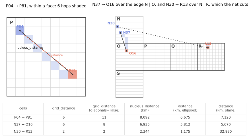
Fig. 15 Three measures between two cells. grid_distance counts hops over
the grid (the shaded path), nucleus_distance is the great circle
between the nuclei (the solid line) and distance the least gap
between the boundaries (dashed). On the right the same measures cross
face edges: between N and O, which the net keeps together, and between
N and R, which the net cuts, so that cells two hops apart on the cube
lie at opposite ends of the plane. The table gives each measure for
the three pairs.
In a DGGS, joins by containment or overlap are operations on identifiers: a prefix comparison or a lookup. Proximity queries are not: finding the nearest neighbour, the cells within 5 km of a road, or the pairs closer than a threshold. A k-ring gives the candidates, but ranking or filtering them needs a distance per pair, and a distance on the ellipsoid is an iterative geodesic calculation. Bowater and Stefanakis [BS2019] list distance and direction from the identifiers alone among the open questions for rHEALPix, after Sirdeshmukh [Sird2018]. The package offers one exact grid measure, two closed-form approximations with stated error bounds, and the exact geodesic as an option on each.
The measures
Measure |
What it is |
Error and cost |
|---|---|---|
The number of hops between two cells over the cube: the smallest
|
Exact as a count, by integer arithmetic on the identifiers; about 10 µs. As a length, see below. |
|
The great circle between the nuclei on the authalic sphere, where the projection’s closed-form inverse lands. |
Within 0.112 % of the ellipsoidal geodesic at every distance; 2 µs
per pair in batch, 76 µs per |
|
The initial bearing between the nuclei, clockwise from north. |
Within 0.064° at short range and 0.1° up to 5,000 km, a few
degrees beyond, and undefined near the antipode, as the geodesic’s
own azimuth is. |
|
The least distance between the cells’ boundaries: 0 when they
touch or nest. On the ellipsoid ( |
Exact on the ellipsoid, at about 5 ms. In the plane 71 µs, but 0.88 to 1.37 times the geodesic on an equatorial face, 0.70 to 1.69 on a polar face, and wrong across the seams of the unfolding. |
Which to use
For a grid question, use the grid measure. “Is this cell within three
cells of that one” is grid_distance(other) <= 3, which is exact,
needs no geometry, and agrees with k_ring. The hop count is also the
right measure for anything defined on the grid, such as a buffer of
k rings or a filter on hops.
For a question in metres, such as filtering or ranking the candidates
from a k-ring against a threshold, use nucleus_distances. Its error
of 0.112 % is small next to the approximation already made by comparing
cells centre to centre: at resolution 8 a cell is about 1.5 km wide,
while the error on a 100 km distance is 110 m. Because the measure is
nucleus to nucleus, two cells that touch have a positive distance of
roughly a cell width, and at coarse resolutions the choice of points
outweighs the choice of surface: in the table of the first figure the
nuclei of P04 and P81 are 8,092 km apart and their boundaries
6,675 km, a cell diagonal’s difference, while the plane and the
ellipsoid differ by a few hundred km and the sphere and the geodesic by
3 km. For a result within the accuracy of the geodesic,
pass exact=True, which runs pyproj.Geod on the same nuclei. Most
of the saving over Cell.distance comes from computing the nuclei in
bulk rather than from the spherical formula, so the exact form is still
fast in batch.
For the gap between two cells’ edges, use Cell.distance on the
ellipsoid. This measure alone is 0 for touching cells and positive
otherwise, and the result is exact, but at 5 ms a pair the method suits
a few pairs rather than a proximity query.
Ranking a k-ring
A proximity query starts from the candidates a k-ring gives and ranks or
filters them by distance. Around N674, a resolution 3 cell near the
edge of the north polar face, the ring of three hops holds 48 cells:
>>> from rhealpixdggs.dggs import WGS84_003
>>> from rhealpixdggs.rhp_wrappers import k_ring
>>> ring = k_ring('N674', 3)
>>> distances = WGS84_003.nucleus_distances(['N674'], ring)
>>> [ring[i] for i in distances.argsort()[1:4]]
['N675', 'N673', 'N672']
>>> int((distances[1:] < 800e3).sum())
14
The hop count orders the candidates only coarsely. The cells of ring 3
start at 735 km from N674 and those of ring 2 reach 1,183 km,
because a hop along a row is shorter than one along a diagonal, and
because the plane’s scale varies across a polar face: the rings
interleave when ranked by distance.
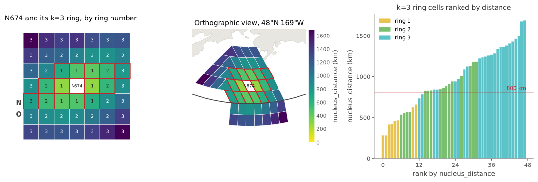
Fig. 16 The 3-ring around N674 ranked by nucleus_distances. Left, the
ring in the plane with each cell’s hop count and its distance as
colour; middle, the same cells on the globe, where the three rows in
face N are stretched and skewed and the rows in O are not; right, the
cells in order of distance, coloured by ring. Ring 3 begins before
ring 2 ends, and two cells of ring 1 come after four of ring 2.
The error of the sphere measures
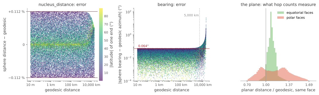
Fig. 17 The sphere measures against the WGS84 geodesic on 400,000 random
pairs, from docs/proximity_error.py. The distance error never
exceeds a / R_A - 1, and shrinks towards the poles; the bearing
error grows only past a few thousand kilometres. Right, how far the
plane stretches distances within a face, which hop counts inherit.
The authalic sphere has the ellipsoid’s area, so the rHEALPix projection
is equal-area on it and its inverse is a closed form: a cell’s nucleus
comes out of the identifier as a longitude and an authalic latitude in
a few arithmetic operations (nuclei()
with authalic=True). A great circle on that sphere differs from the
ellipsoidal geodesic by the scale between the two surfaces, which lies
between b / R_A along a meridian and a / R_A along the equator.
The distance error is therefore bounded by a / R_A - 1, 0.112 % on
WGS84, reached east-west at the equator, and this bound holds at every
distance. The bearing error at short range is half the largest angular
distortion of the same map, 0.064°. The bearing error grows with
distance because a long great circle and a long geodesic between the
same ends leave at different angles, and near the antipode neither has
a meaningful azimuth.
Hop counts as lengths
A hop count is a grid measure. Multiplied by the cell width, the count
approximates a length, with two sources of error. First, a hop is a cell
width along a row or column but longer along a diagonal: the Chebyshev
count is up to 29 % under the straight planar distance (along a
diagonal), the Manhattan count up to 41 % over, and the octile
combination chebyshev + (sqrt(2) - 1) * min(dr, dc) within 8.2 %.
Second, the plane is equal-area, not equidistant: within one face a
planar distance is 0.88 to 1.37 times the geodesic on an equatorial face
and 0.70 to 1.69 times on a polar face (right panel above), and across a
face edge the two faces meet at different scales. Together these put a
hop count times a cell width within a factor of about two of the surface
distance. Where a length is wanted, nucleus_distance costs a few
operations more and is within 0.112 %.
Why there is no exact distance from the identifiers
An identifier is a coordinate: its digits fix a square in the plane,
and the inverse projection is closed form, so computing the nucleus
costs a few operations. But no map from a curved surface to a plane
preserves all distances, so no measure computed from the planar
positions alone can be an exact surface distance. Such a measure is
either a grid metric, exact as a count of hops, or an approximation
whose error depends on where the cells are. The package does not avoid
coordinates; the package avoids the iterative ellipsoidal solver, by
stopping at the authalic sphere within the bound above, and provides the
geodesic through exact=True for results within the accuracy of the
geodesic.