Choosing N_side
N_side is the number of children along each side of a cell: every
cell divides into N_side by N_side children at the next
resolution. The presets WGS84_003 and WGS84_002 are the same
projection on the same ellipsoid with N_side 3 and 2, and everything
in this manual applies to both unless a page says otherwise. This page is
what differs. Values above 3 are discussed at the end.
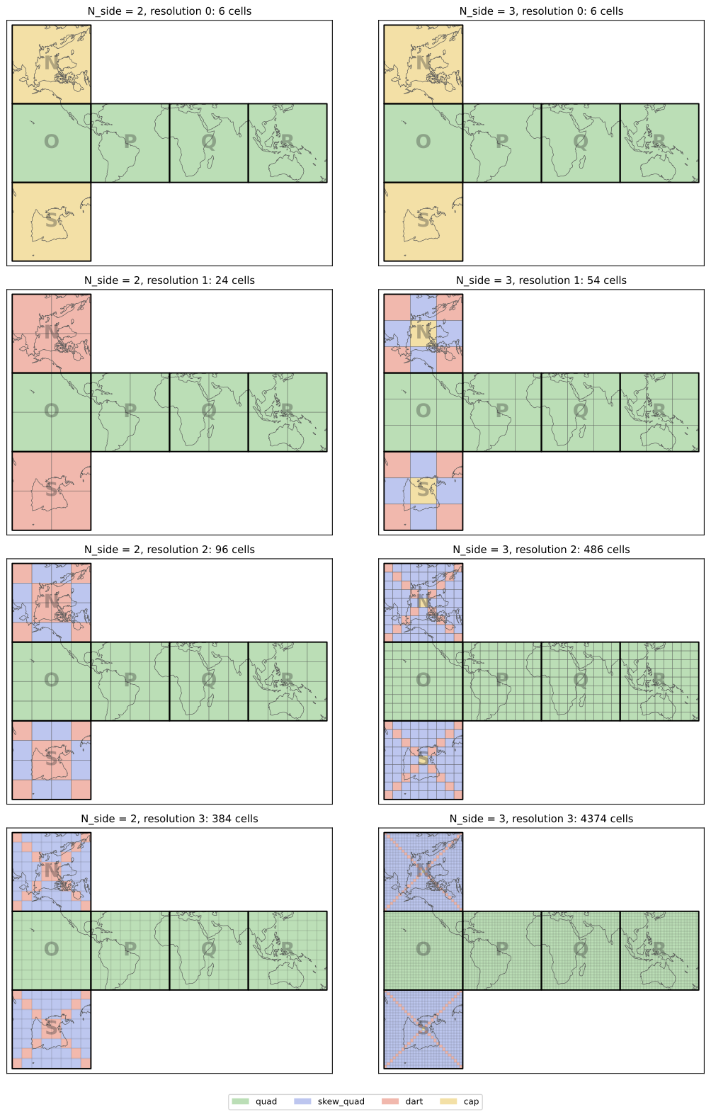
Fig. 9 Resolutions 0 to 3 on both grids. The base cells are the same; from
resolution 1 the grids part ways. With N_side 2 no cell is centred
on the pole, so the pole is a shared vertex of four dart cells and skew
quads only appear at resolution 2. With N_side 3 the centre child
of each polar face is a cap cell containing the pole, at every
resolution.
Refinement and encoding
N_side 2 is one-to-four refinement, N_side 3 one-to-nine. Each
level of an identifier is one digit: 0 to 3 for N_side 2, which is
exactly 2 bits, and 0 to 8 for N_side 3, which needs 4 bits of which
7 of the 16 values are never used. So an N_side 2 identifier packs
into a binary word with no waste, and reaches a given cell size in more,
smaller steps: each level quarters the cell area rather than dividing it
by nine, which gives a finer choice of scales.
The default max_areal_resolution of one square metre sets the finest
resolution of a grid, the first at which cells are smaller than that:
>>> from rhealpixdggs.dggs import WGS84_002, WGS84_003
>>> WGS84_002.max_resolution, WGS84_003.max_resolution
(24, 15)
>>> round(WGS84_002.cell_area(24, plane=False), 3), round(WGS84_003.cell_area(15, plane=False), 3)
(0.302, 0.413)
Reaching one square metre takes 24 levels of 2 bits, 48 bits, with
N_side 2, against 15 levels of 4 bits, 60 bits, with N_side 3.
Shapes and poles
The base cells are the same on both grids: N and S are caps and
O, P, Q and R are quads. From resolution 1 on they part
ways. With odd N_side the centre child of a polar cell is again
centred on the pole, so every resolution has two cap cells; with even
N_side no child is centred, the pole becomes a vertex shared by four
cells, and there are no caps at resolution 1 or finer. Skew quads first
appear at resolution 1 with N_side 3 and at resolution 2 with
N_side 2:
>>> from collections import Counter
>>> def shapes(rdggs, resolution):
...     return dict(sorted(Counter(c.ellipsoidal_shape for c in rdggs.grid(resolution)).items()))
>>> shapes(WGS84_002, 1)
{'dart': 8, 'quad': 16}
>>> shapes(WGS84_002, 2)
{'dart': 16, 'quad': 64, 'skew_quad': 16}
>>> shapes(WGS84_003, 1)
{'cap': 2, 'dart': 8, 'quad': 36, 'skew_quad': 8}
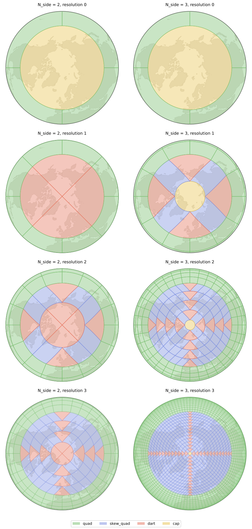
Fig. 10 Resolutions 0 to 3 from above the north pole. On the N_side 2 grid
the four cells at the pole carry it as a vertex, and the GeoJSON export
writes that vertex as a segment along the pole latitude (see
Export).
Because even N_side has no centre child,
rhp_to_center_child() returns None on
such a grid, with a warning:
>>> import warnings
>>> from rhealpixdggs.rhp_wrappers import rhp_to_center_child
>>> rhp_to_center_child('P0', dggs=WGS84_003)
'P04'
>>> with warnings.catch_warnings():
...     warnings.simplefilter('ignore')
...     print(rhp_to_center_child('P0', dggs=WGS84_002))
None
Isolatitude rings
Both grids have the isolatitude property of Isolatitude Rings: nuclei lie
on rings of constant latitude, equally spaced in longitude. The ring
counts and populations differ, as the even-n column of the ring table
there gives: with n cells per base-cell side there are 2n + 1
rings for odd n and 2n for even n, the innermost ring of an
even grid holding the four cells around the pole rather than one cap:
>>> WGS84_002.ring_table(1).population.tolist()
[4, 8, 8, 4]
>>> WGS84_003.ring_table(1).population.tolist()
[1, 8, 12, 12, 12, 8, 1]
The ring-profile figure on the isolatitude page plots an N_side 2 and
an N_side 3 grid together.
Side by side
On WGS84 with the default one square metre floor:
|
|
|
|---|---|---|
refinement |
one to four |
one to nine |
bits per level |
2, all values used |
4, 7 of 16 unused |
digits per level |
one, 0 to 3 |
one, 0 to 8 |
cells at resolutions 1, 2, 3 |
24, 96, 384 |
54, 486, 4374 |
cell width at resolutions 1, 2, 3 |
5004, 2502, 1251 km |
3336, 1112, 371 km |
cell area at resolutions 1, 2, 3 |
21.3, 5.31, 1.33 million km² |
9.45, 1.05, 0.117 million km² |
isolatitude rings at resolutions 1, 2, 3 |
4, 8, 16 |
7, 19, 55 |
shapes at resolution 1 |
quad, dart |
quad, dart, skew quad, cap |
skew quads first appear |
resolution 2 |
resolution 1 |
cell centred on the pole |
resolution 0 only |
every resolution |
centre child |
none |
digit 4 |
finest resolution (cells under 1 m²) |
24, cells of 0.30 m² |
15, cells of 0.41 m² |
bits to encode a finest cell |
48 |
60 |
>>> [6 * 2 ** (2 * k) for k in (1, 2, 3)], [6 * 3 ** (2 * k) for k in (1, 2, 3)]
([24, 96, 384], [54, 486, 4374])
>>> [round(WGS84_002.cell_width(k) / 1000) for k in (1, 2, 3)]
[5004, 2502, 1251]
>>> [round(WGS84_003.cell_width(k) / 1000) for k in (1, 2, 3)]
[3336, 1112, 371]
>>> [round(WGS84_002.cell_area(k, plane=False) / 1e12, 2) for k in (1, 2, 3)]
[21.25, 5.31, 1.33]
>>> [round(WGS84_003.cell_area(k, plane=False) / 1e12, 3) for k in (1, 2, 3)]
[9.446, 1.05, 0.117]
>>> [len(WGS84_002.ring_table(k).population) for k in (1, 2, 3)]
[4, 8, 16]
>>> [len(WGS84_003.ring_table(k).population) for k in (1, 2, 3)]
[7, 19, 55]
Which to choose
N_side 3 keeps a cell centred on every pole and a centre child under
every parent, which some hierarchical algorithms rely on, and its coarse
levels are the ones the rHEALPix literature describes. N_side 2 gives
compact binary identifiers and twice as many scales to choose from between
the same coarsest and finest cells, at the price of four cells meeting at
each pole. Both are exact, equal-area, congruent hierarchies, and every
operation in this package accepts either.
Larger values
Index strings, a face letter followed by one digit per resolution, are
defined for N_side 2 and 3, the grids whose digits are single
characters; has_index_strings
says so, and parse_index() and
format_index() are the one place
that reads and writes them. A grid with a larger N_side can be
constructed and used through the tuple-based
Cell API, but every function that takes or
returns index strings raises ValueError for it, and str(cell)
gives a display form such as '(N, 10, 15)' that is not an identifier.
Two grids share cells above resolution 0 only when their N_side values
are powers of one base: N_side 4 is the N_side 2 grid restricted to
even resolutions, 9 is the 3 grid likewise, while 5, 7 and 11 partition
the cube in ways no other grid does. The general rule, decided in issue
#146 and to be implemented with the mixed-aperture grids of issue #169,
treats a grid as a sequence of prime apertures, one per level, and writes
an identifier as a face letter followed by one digit per prime level, each
digit with the width its prime needs; an N_side 4 cell then carries
its N_side 2 identifier, so composite grids never need identifiers of
their own.