Isolatitude Rings

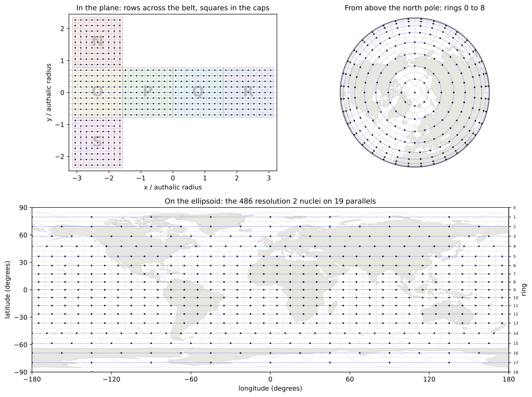
Fig. 11 The nuclei of the resolution 2 cells of the (0, 0)-rHEALPix DGGS on WGS84, with a line through each ring. Rows and concentric squares in the plane become parallels of latitude on the ellipsoid, and along each one the nuclei are equally spaced in longitude.

The property

The nucleus of a cell is the point of the ellipsoid under the centre of its planar square. In the equatorial belt the rHEALPix projection maps parallels of latitude to horizontal lines, so the nuclei of a row of cells, which share a planar y, share a latitude, and the row runs right across the four equatorial faces O, P, Q and R. In each polar cap the projection maps parallels to squares concentric with the cap’s centre, so the cells at a given Chebyshev distance from the pole cell share a latitude too. The nuclei of a resolution therefore lie on a small number of isolatitude rings: 2n + 1 of them for n = 3 ** k cells per base-cell side at resolution k, against 6 n ** 2 cells. Along each ring the nuclei sit at a constant longitude step, since they are equally spaced in the plane and, on a parallel, planar x is proportional to longitude.

rHEALPix inherits this from HEALPix [GRS2013]; HEALPix is the Hierarchical Equal Area isoLatitude Pixelization, and rHEALPix is its rearranged form. In HEALPix it is the reason the grid exists: a spherical harmonic transform evaluates the associated Legendre functions once per ring rather than once per cell, and handles the longitude direction on each ring with a fast Fourier transform, which brings the cost of a transform down from the square of the cell count to about its three-halves power [Gorski2005]. rHEALPix keeps the rings and the equal spacing while changing the ring populations, so software written for HEALPix’s layout does not apply directly; what this package provides is the ring structure itself, described below, from which such a transform can be laid out.

The ring table

Write \(n = N_{side}^k\) for the number of cells along a base cell’s side at resolution \(k\), and \(q = \lceil n / 2 \rceil\) for the number of rings in each polar cap. Rings are numbered from 0 at the north pole to \(n + 2q - 1\) at the south pole, and their nucleus latitudes \(\beta\) on the authalic sphere are:

Region	Ring	Cells on ring	\(\sin \beta\)
North cap, Chebyshev distance \(m = 0, \dots, q - 1\) from the pole cell	\(m\)	\(8m\) (odd \(n\); 1 when \(m = 0\)), \(8m + 4\) (even \(n\))	\(1 - \sigma^2 / 3\), with \(\sigma = 2m / n\) (odd) or \((2m + 1) / n\) (even)
Equatorial belt, row \(r = 0, \dots, n - 1\)	\(q + r\)	\(4n\)	\(\tfrac{2}{3} \left( 1 - \tfrac{2r + 1}{n} \right)\)
South cap, Chebyshev distance \(m\)	\(q + n + (q - 1 - m)\)	as the north cap	as the north cap, negated

For odd \(n\) the pole cell is a ring of its own; for even \(n\) the four cells around the pole form the innermost ring. On the equatorial rings the first nucleus is at longitude \(-180° + 45°/n\) and the step is \(90°/n\); on a cap ring with \(8m\) (or \(8m + 4\)) cells the first nucleus is at \(-180°\) and the step is \(90° / (2m)\) (or \(90° / (2m + 1)\)). The longitudes are the same on the ellipsoid and the authalic sphere; the latitudes are not, and the ellipsoidal nucleus latitude \(\phi\) follows from \(\beta\) by the inverse authalic latitude conversion.

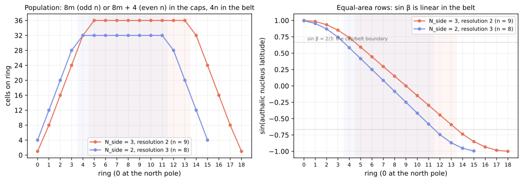
Fig. 12 The ring table for odd and even \(n\). The population grows by 8 per ring through a cap and is constant across the belt; the odd grid starts from a single pole cell, the even grid from four. The sine of the nucleus latitude is linear in ring number through the belt, which is the equal-area property: each row of cells covers the same band of \(\sin \beta\).

All of this is arithmetic on the index digits and the resolution; no projection is involved. The ring of a cell follows from its row and column within its base cell, which are the base-\(N_{side}\) numbers formed from the row and column parts of its digits.

Reading the rings from the API

Cell.ring gives a cell’s ring number, and RHEALPixDGGS.rings the same for many index strings at once. Cells on one ring share a nucleus latitude whatever their base cell:

>>> from rhealpixdggs.dggs import WGS84_003
>>> rdggs = WGS84_003
>>> [rdggs.cell(suid).ring() for suid in (['N', 4], ['N', 0], ['P', 4], ['S', 8])]
[0, 1, 3, 5]
>>> rdggs.rings(['O0', 'P0', 'Q0', 'R0']).tolist()
[2, 2, 2, 2]
>>> {round(float(rdggs.cell([face, 0]).nucleus(plane=False)[1]), 6) for face in 'OPQR'}
{26.490119}

RHEALPixDGGS.ring_table describes every ring of a resolution: its population, the latitude its nuclei share (on the ellipsoid and on the authalic sphere), and the longitude of its first nucleus and the step to the next. This is the whole of resolution 1:

>>> table = rdggs.ring_table(1)
>>> table.population.tolist()
[1, 8, 12, 12, 12, 8, 1]
>>> table.latitude.round(3).tolist()
[90.0, 58.528, 26.49, 0.0, -26.49, -58.528, -90.0]
>>> table.authalic_latitude.round(3).tolist()
[90.0, 58.414, 26.388, 0.0, -26.388, -58.414, -90.0]
>>> table.first_longitude.tolist()
[nan, -180.0, -165.0, -165.0, -165.0, -180.0, nan]
>>> table.longitude_spacing.tolist()
[nan, 45.0, 30.0, 30.0, 30.0, 45.0, nan]

RHEALPixDGGS.cells_on_ring is the inverse of rings: the index strings of one ring, in increasing nucleus longitude from first_longitude. The cells of a cap ring walk around the pole cell; the cells of an equatorial ring run across the four faces:

>>> rdggs.cells_on_ring(1, 1).tolist()
['N6', 'N7', 'N8', 'N5', 'N2', 'N1', 'N0', 'N3']
>>> rdggs.cells_on_ring(1, 2).tolist()
['O0', 'O1', 'O2', 'P0', 'P1', 'P2', 'Q0', 'Q1', 'Q2', 'R0', 'R1', 'R2']
>>> rdggs.nuclei(rdggs.cells_on_ring(1, 2)).round(3)[:4].tolist()
[[-165.0, 26.49], [-135.0, 26.49], [-105.0, 26.49], [-75.0, 26.49]]

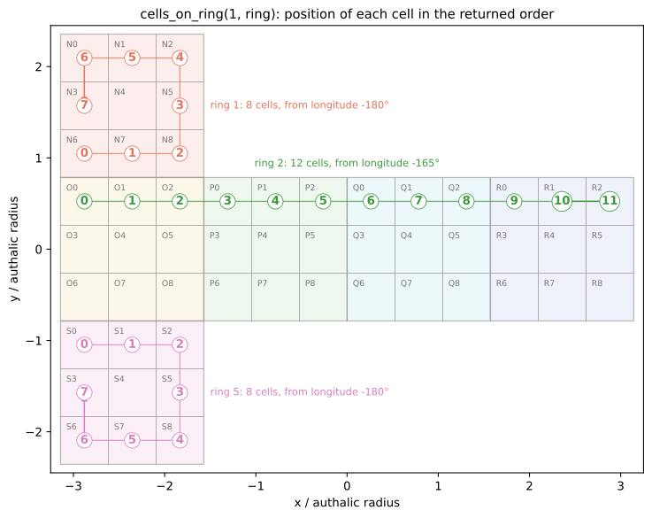
Fig. 13 The order cells_on_ring returns: increasing nucleus longitude from the ring’s first_longitude. In the plane that is left to right along an equatorial row, anticlockwise around the north pole cell and clockwise around the south.

Together they lay out a per-ring loop. The longitude direction on each ring is a discrete Fourier transform of the values in cells_on_ring order. Sampling the field \(\cos\phi \cos\lambda\), which has a single longitudinal wavenumber, the transform of each ring holds one nonzero coefficient, at wavenumber 1, of size \(\cos\phi / 2\):

>>> import numpy as np
>>> table = rdggs.ring_table(2)
>>> for ring in (1, 4, 9, 13):
...     lon, lat = np.radians(rdggs.nuclei(rdggs.cells_on_ring(2, ring))).T
...     spectrum = np.abs(np.fft.rfft(np.cos(lat) * np.cos(lon))) / len(lon)
...     print(ring, spectrum.argmax(), spectrum.max().round(6),
...           (np.cos(lat[0]) / 2).round(6), np.delete(spectrum, 1).max().round(12))
1 1 0.089957 0.089957 0.0
4 1 0.337328 0.337328 0.0
9 1 0.5 0.5 0.0
13 1 0.402116 0.402116 0.0

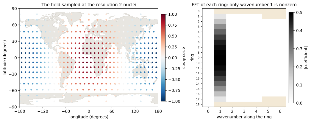
Fig. 14 The same field and the magnitude of its Fourier coefficients along each ring. One column is lit because the field has a single longitudinal wavenumber; it fades towards the poles with \(\cos\phi\). A ring of \(c\) cells resolves wavenumbers up to \(c / 2\), so the short polar rings have fewer coefficients.

The Legendre part of a transform, which combines the rings, depends only on each ring’s latitude, so it is evaluated once per row of the table rather than once per cell.

What the rings give you, and what they do not

The rings and the equal spacing along them are what make a fast transform possible, and ring_table and cells_on_ring supply exactly the description such a transform needs: a latitude, a population, a first longitude and an offset for each ring. Three qualifications:

• Use the authalic latitude. Spherical harmonics live on a sphere, and the sphere on which the rHEALPix cells are equal-area, and the rings sit exactly where the table above says, is the authalic sphere. Feed a transform authalic_latitude, not latitude. On a spherical grid the two coincide.

• Analysis is approximate. Equal-area cells make equal weights the natural quadrature, but the rings are not at Gauss-Legendre latitudes, so recovering coefficients from values on the grid is not exact, and is done iteratively in practice, as it is for HEALPix. Along an equatorial ring of 4n cells the Fourier transform resolves wavenumbers up to 2n, so that is roughly the highest degree a resolution supports before aliasing.

• The rings are not a transform. A transform combines the rings with the associated Legendre functions and, for analysis, iterates. That work is borrowed from ducc0, whose ring-based routines take exactly the columns of ring_table: Spherical Harmonics wraps them for the nuclei of a grid, with the optional harmonics extra installed. healpy’s map2alm and alm2map cannot be used instead: they assume HEALPix’s ring populations.